Computational Physics Essentials
Bridging Theory and Simulation in Modern Physics
How do physicists predict the behavior of systems too complex for pencil-and-paper mathematics?
222 pages10 chaptersApr 5, 2026Computational Physics
About this book
Computational physics has become indispensable for modern theoretical research, yet many practitioners struggle to connect fundamental concepts with practical implementation. This book bridges that gap by teaching you how to translate physical theories into working simulations. You'll explore the essential numerical methods that power contemporary physics research—from solving differential equations to simulating particle systems—while understanding the mathematical foundations and practical limitations of each approach. Rather than overwhelming you with code, this guide emphasizes the physics-first perspective: why certain methods work, when they fail, and how to validate your results. Whether you're studying quantum mechanics, classical dynamics, or field theory, you'll gain the conceptual framework and practical skills to build reliable simulations that advance your understanding of the physical world.
Table of contents
- IntroductionWhy Computational Physics Matters, From Theory to Simulation, How to Use This BookRead below
- Chapter 1: Foundations of Computational PhysicsThe Computational Paradigm in Physics, Discretization: From Continuous to Discrete, Understanding Error Sources
- Chapter 2: Essential Numerical MethodsSolving Ordinary Differential Equations, Tackling Partial Differential Equations, Solving Linear Systems Efficiently, Root Finding and Optimization
- Chapter 3: Classical Dynamics and MechanicsSimulating Particle Systems, Integration Schemes and Stability, Modeling Forces and Interactions
- Chapter 4: Quantum Systems and Wave FunctionsSolving the Schrödinger Equation, Eigenvalue Problems in Quantum Mechanics, Time-Dependent Wave Function Evolution
- Chapter 5: Field Theory and Continuum SimulationsDiscretizing Fields on Grids, Finite Difference Methods, Spectral Methods for Field Equations
- Chapter 6: Stochastic Methods and Monte CarloRandom Sampling and Probability, Monte Carlo Integration Techniques, Molecular Dynamics and Ensemble Methods
- Chapter 7: Validation, Verification, and BenchmarkingTesting and Validation Strategies, Convergence Analysis and Accuracy, Comparing with Experimental Data
- Chapter 8: Computational Efficiency and OptimizationChoosing the Right Algorithm, Performance Tuning and Profiling, Parallel Computing Fundamentals
- Chapter 9: Advanced Topics and Emerging MethodsMachine Learning in Physics Simulations, Adaptive and Multiscale Methods, GPU Computing for Physics
- Chapter 10: Case Studies: From Theory to ImplementationCase Study 1: Planetary Orbital Mechanics, Case Study 2: Quantum Harmonic Oscillator, Case Study 3: Fluid Dynamics Simulation
- ConclusionSynthesizing Computational and Theoretical Physics, Future Directions in Computational Physics
- Glossary of Key Terms
- Further Reading and Resources
Introduction
Physics has always been a discipline built on the tension between what we can imagine and what we can calculate. For centuries, the tools available to physicists were limited to pencil, paper, and the occasional mechanical calculator. Those constraints shaped the kinds of problems that could be solved and, by extension, the kinds of questions that were even worth asking. The arrival of digital computers in the mid-twentieth century changed that equation permanently. Suddenly, problems that had been analytically intractable became approachable, and entire new branches of physics opened up as a result.
Today, computational physics sits at the heart of nearly every active research frontier. Whether scientists are modeling the collision of neutron stars, predicting the folding behavior of proteins, or simulating the early universe, they are relying on numerical methods running on powerful hardware. This is not a niche specialty reserved for a small group of experts. It is a core skill set that any serious physics student or practitioner needs to develop. The gap between knowing the theory and being able to simulate it is real, but it is also bridgeable with the right conceptual foundation.
This book is designed to help you cross that gap. It does not assume you are already a programmer, nor does it assume you have forgotten all your physics. It assumes you have a working knowledge of classical mechanics, some exposure to differential equations, and a genuine curiosity about how physical theories translate into working simulations. From that starting point, the chapters ahead will build your understanding of numerical methods, simulation design, error analysis, and validation in a way that keeps the physics front and center throughout.
One important note before diving in: this book is deliberately physics-first rather than code-first. You will encounter pseudocode, algorithmic descriptions, and mathematical formulations throughout, but the emphasis is always on understanding why a method works, when it is appropriate, and what its limitations are. The specific programming language you use to implement these ideas is secondary to understanding the ideas themselves. Python, C++, Julia, and Fortran are all used in active physics research, and the concepts here apply across all of them.
Why Computational Physics Matters
The most honest answer to the question of why computational physics matters is simple: most physically interesting problems cannot be solved analytically. The hydrogen atom has a clean closed-form solution. The helium atom does not. Add one more electron, and the exact mathematics becomes impossible to write down in a finite number of steps. This is not a failure of human ingenuity. It is a fundamental feature of systems with many interacting parts, and it applies across every branch of physics from condensed matter to cosmology.
Consider a few concrete examples that illustrate the scope of this challenge. In classical mechanics, the two-body gravitational problem has an elegant analytical solution that Kepler and Newton worked out centuries ago. The three-body problem, however, is generally chaotic and has no closed-form solution for arbitrary initial conditions.[1] Simulating the solar system accurately over millions of years requires numerical integration. In quantum mechanics, density functional theory calculations that predict the electronic structure of materials involve solving coupled equations for hundreds or thousands of electrons simultaneously. No analytical shortcut exists for those systems.
Beyond simply solving equations that resist analytical treatment, computational physics enables a qualitatively different kind of scientific exploration. Simulations allow researchers to run controlled experiments that would be physically impossible or prohibitively expensive in a laboratory. You can simulate a supernova, vary the initial mass of the star, and observe how the outcome changes. You can model a material at temperatures and pressures that no lab on Earth can sustain. This predictive and exploratory power has made computational methods an essential third pillar of physics alongside theory and experiment.
The practical impact of this is visible in major scientific achievements of recent decades. The detection of gravitational waves by LIGO in 2015 depended critically on numerical relativity simulations that predicted the waveform signatures of merging black holes.[2] Without those computational templates, the signal could not have been identified in the detector noise. Similarly, the Standard Model predictions tested at the Large Hadron Collider rely on Monte Carlo simulations of particle interactions that run on massive computing clusters. Computation is not a support tool for these discoveries. It is a central part of the scientific method itself.
For students and early-career researchers, the practical value of computational skills is equally significant. Employers in academia, national laboratories, and industry consistently rank programming and numerical methods among the most sought-after skills in physics graduates.[3] Learning to build and validate simulations is not just intellectually rewarding. It is a direct investment in your ability to contribute to modern research and to work effectively across the increasingly interdisciplinary landscape of contemporary science.
There is also a deeper conceptual benefit that often goes unmentioned. Writing a simulation forces you to understand a physical theory at a level of precision that reading about it never quite demands. When you implement the Euler method for a simple harmonic oscillator and watch it spiral outward instead of oscillating stably, you learn something visceral about numerical stability that no textbook description fully conveys. The act of translating physics into an algorithm exposes assumptions, approximations, and subtleties that remain invisible when you only work with equations on paper.
Computational physics also plays a growing role in education itself. Interactive simulations have transformed how students visualize phenomena like wave interference, orbital mechanics, and phase transitions. Tools like PhET Interactive Simulations from the University of Colorado have demonstrated that well-designed computational visualizations significantly improve conceptual understanding in physics courses.[4] Understanding how those simulations work puts you in a position not just to use them, but to build and improve them.
Key takeaway: Computational physics is not a workaround for hard problems. It is a fundamental scientific methodology that enables discoveries, tests theories, and builds understanding in ways that purely analytical approaches cannot match.
From Theory to Simulation
The journey from a physical theory to a working simulation involves several distinct steps, and understanding each one is essential for building reliable results. Many beginners treat this process as a single leap: take the equation, write some code, run it, and look at the output. In practice, each step introduces its own challenges and potential sources of error. Recognizing the structure of this process is the first step toward doing it well.
The process generally follows this sequence:
- Identify the physical model. What equations govern the system? What assumptions are built into those equations?
- Choose a mathematical formulation. Should you work with differential equations, integral equations, or an energy-based variational principle?
- Select a numerical method. Which algorithm is appropriate for this type of equation, given your accuracy requirements and available resources?
- Discretize the problem. Convert continuous variables into discrete representations that a computer can process.
- Implement and test. Write the algorithm, verify it against known solutions, and check for bugs.
- Validate the results. Compare outputs against analytical benchmarks, experimental data, or established simulations.
- Interpret and communicate. Extract physical meaning from the numerical output and present it clearly.
Each of these steps deserves careful attention. The first step, identifying the physical model, is often underestimated. Every model is an approximation of reality, and the approximations you accept at the start propagate through everything that follows. For example, if you model air resistance as purely linear in velocity when the actual drag is quadratic at high speeds, your simulation will produce systematically wrong results no matter how accurate your numerical method is. The physics of the model matters more than the sophistication of the algorithm.
Discretization deserves special emphasis because it is where continuous mathematics meets the finite world of digital computation. A differential equation describes how a quantity changes at every point in a continuous space or time. A computer can only store and process a finite number of values. The process of converting one into the other, choosing a grid spacing, a time step, or a basis set, introduces discretization error. This error can be controlled and reduced, but it can never be entirely eliminated. Understanding how it behaves is central to trusting your results.
A concrete example helps make this tangible. Suppose you want to simulate the motion of a pendulum. The governing equation is a second-order nonlinear ordinary differential equation. You cannot solve it exactly for large angles, so you turn to numerical integration. You choose a time step of 0.1 seconds and apply the simple Euler method. After a few oscillations, you notice the amplitude is growing, which is physically wrong for a frictionless pendulum. The energy should be conserved. What went wrong? The Euler method is not symplectic, meaning it does not preserve the geometric structure of Hamiltonian systems, and it systematically injects energy into the simulation. Switching to the Verlet method, which is symplectic, fixes the problem. This is a perfect illustration of why algorithm selection is a physics decision, not just a technical one.
The validation step is equally critical and equally easy to skip when you are eager to see results. A simulation that produces plausible-looking output is not necessarily a correct simulation. The standard practice is to test your code against cases where the answer is known exactly. For the pendulum, you can verify the small-angle limit against the analytical solution for simple harmonic motion. If your simulation matches that limit to within expected numerical precision, you have evidence that the implementation is correct. Only then should you trust results in the regime where no analytical solution exists.
It is also worth recognizing that the translation from theory to simulation is not a one-way street. Running simulations often reveals unexpected behavior that prompts you to revisit the physical model. You might discover that a term you neglected is actually important, or that a symmetry you assumed is broken in certain parameter regimes. This feedback loop between simulation and theory is one of the most productive aspects of computational physics. The simulation is not just a calculator. It is a tool for developing physical intuition.
Example workflow: Simulating heat diffusion in a metal rod
Physical model: The heat equation, a parabolic partial differential equation. Discretization: Replace the spatial derivative with finite differences on a uniform grid; use a time-stepping scheme for the temporal derivative. Method selection: Explicit Euler for simplicity, or Crank-Nicolson for better stability. Validation: Compare the numerical solution at early times against the known analytical solution for a Gaussian initial temperature profile. Once validated, extend to geometries or boundary conditions that have no analytical solution.
The tools available for this workflow have expanded dramatically in recent years. Scientific computing libraries in Python (NumPy, SciPy), Julia, and C++ provide robust, well-tested implementations of many standard numerical methods. This means you rarely need to implement a basic ODE solver from scratch. What you do need is a clear understanding of what those solvers are doing, what their assumptions are, and when they are appropriate. That understanding is what this book is designed to provide.
Finally, it is worth acknowledging that the path from theory to simulation is rarely linear in practice. Real research involves iteration, dead ends, and unexpected discoveries. A method that works beautifully for one problem may fail completely for a slightly different one. Building the judgment to recognize these situations, and the toolkit to respond to them, is the real goal of learning computational physics. The specific algorithms are important, but the deeper skill is knowing how to think about the problem.
How to Use This Book
This book is organized to build your understanding progressively, starting from foundational concepts and moving toward more specialized and advanced topics. However, it is also designed so that individual chapters can be read independently if you already have background in certain areas. The structure reflects the natural flow of a computational physics project: understand the foundations, learn the methods, apply them to specific physical domains, and then validate and optimize your results.
Here is a brief map of what each part of the book covers:
- Chapter 1 (Foundations): Introduces the computational paradigm, explains discretization, and covers the main sources of numerical error. This chapter is essential reading if you are new to computational methods.
- Chapter 2 (Numerical Methods): Covers the core algorithms you will use repeatedly: ODE solvers, PDE approaches, linear system solvers, and root-finding methods. Think of this as your numerical toolkit.
- Chapters 3 through 6: Apply these tools to specific physical domains: classical dynamics, quantum systems, field theory, and stochastic methods. Each chapter is relatively self-contained and can be read in any order once you have the Chapter 2 foundations.
- Chapter 7 (Validation): Addresses how to test and trust your simulations. This is one of the most practically important chapters in the book.
- Chapter 8 (Optimization): Covers computational efficiency, algorithm selection, and parallel computing. Relevant when your simulations need to scale up.
- Chapter 9 (Advanced Topics): Explores machine learning in physics, adaptive methods, and GPU computing. These are frontier areas that are reshaping the field.
- Chapter 10 (Case Studies): Walks through three complete examples from physical setup to validated simulation, tying together everything from earlier chapters.
If you are a student working through a computational physics course, the recommended path is to read the chapters in order. The progression from foundations to methods to applications mirrors the logical structure of the subject, and later chapters build on concepts introduced earlier. If you are a researcher or practitioner looking to fill specific gaps, you can navigate directly to the relevant chapter. Each chapter includes enough context to be useful on its own, with references back to earlier material where needed.
Throughout the book, you will encounter several recurring features designed to reinforce learning. Worked examples walk through specific calculations or algorithm applications step by step. Common pitfalls highlight mistakes that are easy to make and explain how to avoid them. Conceptual checkpoints pose questions that test whether you have understood the key ideas before moving on. These are not just decorative elements. They reflect the kinds of thinking that experienced computational physicists actually do when approaching a new problem.
On the question of programming language: the examples and pseudocode in this book are written to be language-agnostic wherever possible. When specific syntax is shown, it is chosen for clarity rather than to advocate for any particular language. Python is used in some examples because of its readability and widespread adoption in the physics community, but the underlying algorithms are equally applicable in Julia, MATLAB, C++, or any other scientific computing environment. The goal is always to understand the method, not to memorize a particular implementation.
Mathematics is used throughout the book at the level of undergraduate physics. You should be comfortable with calculus, linear algebra, and basic differential equations. Complex analysis and tensor notation appear in later chapters but are introduced with enough context to be accessible. If you find a particular mathematical concept unfamiliar, the glossary at the back of the book provides concise definitions, and the further reading section points to resources for deeper background.
One of the most valuable things you can do while reading this book is to implement the examples yourself. Reading about the Runge-Kutta method is useful. Watching it conserve energy where Euler fails is genuinely illuminating. Even simple implementations in a notebook or script will deepen your understanding far more than passive reading. The case studies in Chapter 10 are particularly well-suited for this kind of hands-on engagement, as they provide complete problem setups that you can reproduce and then modify to explore variations.
It is also worth setting realistic expectations about what this book covers and what it does not. Computational physics is an enormous field, and no single volume can cover all of it. This book focuses on the core methods and concepts that appear most broadly across physics research. It does not cover specialized topics like lattice QCD, finite element methods for structural mechanics, or the full depth of molecular dynamics force fields. Those topics have excellent dedicated resources, some of which are listed in the further reading section. The goal here is to give you a strong enough foundation that you can approach those specialized resources with confidence.
Finally, approach this material with patience and curiosity. Computational physics rewards persistence. The first time you implement a simulation and see it produce physically meaningful results, there is a genuine sense of satisfaction that comes from having built something that captures a piece of how the universe works. That experience is worth working toward, and every concept in this book is a step in that direction.
A practical suggestion before you begin: Set up a working scientific computing environment before reading Chapter 1. Having Python with NumPy and Matplotlib installed, or an equivalent environment in your preferred language, means you can test ideas immediately as you encounter them. The friction of setting up tools later often interrupts the flow of learning at exactly the wrong moment.
Notes
Introduction
- 1. M. Valtonen and H. Karttunen, The Three-Body Problem, Cambridge University Press, 2006
- 2. Abbott and others, "Observation of Gravitational Waves from a Binary Black Hole Merger," Physical Review Letters, 2016
- 3. American Institute of Physics, Physics Workforce Report, AIP Publishing, 2022
- 4. C. Wieman and others, "PhET: Simulations That Enhance Learning," Science, 2008
This is the end of the free sample. The full book has 10 chapters.
Want this book written for you?
Tell us your goals and background, and get your own version of this book, tailored by AI to you.


Benefits of AI-tailored books
- Read one book, not ten:
- all the Computational Physics knowledge you need, gathered into a single book.
- Save days of learning:
- tell us your goals, choose your topics, and the whole book is built around them.
- Learn effortlessly:
- Computational Physics book written for your specific background and expertise.
- Understand at a glance:
- includes charts, tables, timelines, checklists, decision trees, and more.
- Stay current:
- written the day you order it, not years ago.
- Trust what you read:
- every book is checked for accuracy, with real research when your subject needs it.
Create your unique book in 3 steps
- 1. Select your focus
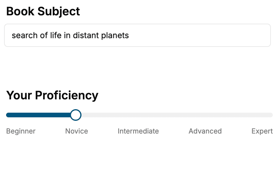
Select the focus of your Computational Physics book and share your background
- 2. Personalize your book
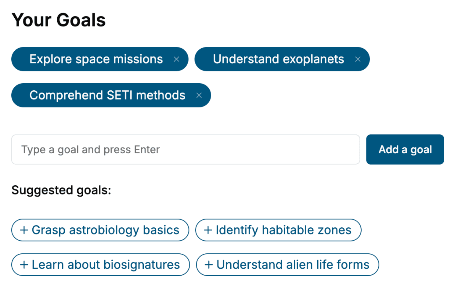
Specify your goals and choose sub-topics to include
- 3. Get your tailored book
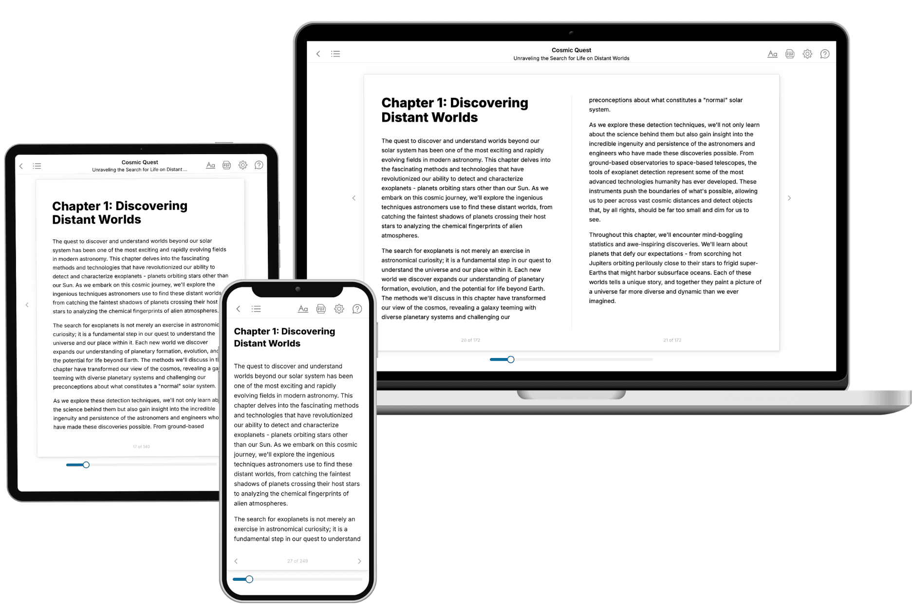
Your book is ready in 10 minutes. Read it online, download as EPUB or PDF, or send to Kindle.
Frequently asked questions
- What is TailoredRead?
TailoredRead creates complete, full-length nonfiction ebooks, written specifically for you. Tell us what you want to learn and why, and TailoredRead writes you a complete ebook on it, with charts, tables, and diagrams throughout. Read it online, on Kindle, or on any e-reader, or download it as a PDF or EPUB. Every book is written fresh the day you order it.
- How is the book tailored to me?
Before anything is written, you answer a few short questions about your goals, your background, and the topics you care about. Your book is then planned around your answers: written at your level, focused on your goals, and covering the topics you chose, instead of the one-size-fits-all book a store sells everyone.
- Will it read like generic AI content?
No. Your book isn't a chat transcript: it's planned chapter by chapter before a single word is written, told in a clear book voice, and explains ideas visually with charts, tables, and diagrams. After writing, every book goes through an editorial pass that polishes chapters so the book reads consistent from start to finish. Judge for yourself: browse thousands of sample books on our Explore Books page.
- How accurate is the content?
Our AI first checks whether your subject needs live research. Niche and fast-moving subjects are researched before writing, and the book plan and chapters are grounded in what it finds. After writing, every book goes through a quality pass that checks its facts and consistency, and researched books list their sources in a Notes section at the back.
- How long is the book?
You choose the length: Comprehensive (250-300 pages), Detailed (150-200 pages), Essential (70-100 pages), or Short (30-50 pages).
- Does the book include visuals?
Yes. Every book includes charts, tables, and diagrams: timelines, checklists, step-by-step guides, decision trees, comparison tables, matrices, and bar charts. A typical book includes dozens of these visual elements.
- Can I read it on Kindle? What formats can I download?
Yes. Every book can be read in our online reader or downloaded as a PDF or EPUB. The EPUB can be opened with Kindle, Apple Books, Kobo, and any e-reader. The Commercial and Author licenses also include an editable Word (DOCX) and Markdown download.
- How much does it cost?
About the price of a regular ebook. The exact price depends on your book's length and complexity, from $2 for the shortest books to $35 for the most comprehensive, and it's shown when you review your book, before you commit to anything. Each book is a one-time purchase, yours to keep, no subscription. Licenses that let you share, teach, or publish your book range from $35.99 to $49.99.
- Can I preview the book before purchasing?
Before you pay, you'll see what your book will cover: the title, a detailed description, the estimated length, and the complete chapter-by-chapter table of contents, so you know what you're getting before you decide. The full text itself is written after you purchase.
- How long does it take to create a book?
About 10 minutes. You can start reading the opening chapters while the rest is still being written.