Hamiltonian Dynamics in Computation
Mastering Energy-Preserving Algorithms for Scientific Computing
Master the mathematical foundations and practical implementation of Hamiltonian dynamics to build numerical algorithms that preserve energy and structure in your simulations.
207 pages8 chaptersJul 23, 2026Computational Physics
About this book
This book bridges the gap between classical mechanics and modern computational science, showing you how Hamiltonian principles lead to more accurate, stable, and efficient algorithms. You'll learn why standard numerical methods fail for long-term simulations and how symplectic integrators solve this problem. Through clear explanations and concrete examples, discover how to apply Hamiltonian dynamics to molecular dynamics, optimization, machine learning, and other computational domains. Whether you're simulating physical systems, training neural networks, or solving differential equations, understanding Hamiltonian dynamics gives you powerful tools to improve accuracy while reducing computational cost. This book equips you with both the theoretical understanding and practical skills needed to implement these advanced techniques in your own work.
Table of contents
- IntroductionWhy Hamiltonian Dynamics Matters in Computing, Limitations of Standard Numerical Methods, How This Book Is Organized, What You Need to KnowRead below
- Chapter 1: Foundations of Hamiltonian MechanicsFrom Newton to Hamilton: A Brief Review, Phase Space and Canonical Coordinates, The Hamiltonian Function and Energy Conservation, Hamilton's Equations of Motion
- Chapter 2: Geometric Structures in Hamiltonian SystemsSymplectic Geometry and Manifolds, Poisson Brackets and Conservation Laws, Liouville's Theorem and Phase Space Volume, Invariant Structures and Their Preservation
- Chapter 3: Numerical Integration MethodsStandard Integrators: Euler, Runge-Kutta, and Beyond, Error Accumulation in Long-Term Simulations, Stability Analysis and Convergence, Comparing Methods: When Standard Approaches Fail
- Chapter 4: Symplectic Integrators: Theory and DesignWhat Makes an Integrator Symplectic, Splitting Methods and Composition, Verlet and Leapfrog Algorithms, Higher-Order Symplectic Integrators
- Chapter 5: Implementing Hamiltonian AlgorithmsPractical Implementation Strategies, Choosing Step Size and Integration Order, Optimizing for Computational Efficiency, Working Code Examples and Patterns
- Chapter 6: Molecular Dynamics and N-Body SimulationsMolecular Dynamics as a Hamiltonian System, Force Fields and Potential Energy Functions, The N-Body Problem and Gravitational Systems, Real-World Applications and Case Studies
- Chapter 7: Hamiltonian Dynamics in OptimizationViewing Optimization Through Hamiltonian Lens, Gradient Descent as Hamiltonian Flow, Accelerated Optimization Methods, Applications to Machine Learning and Neural Networks
- Chapter 8: Advanced Topics and ExtensionsConstrained Hamiltonian Systems, Variational Integrators and Discrete Mechanics, Adaptive and Hybrid Methods, Connections to Quantum Computing and Simulation
- ConclusionKey Takeaways and Synthesis, Future Directions in Hamiltonian Computing, Your Next Steps
- Glossary
- Further Reading and Resources
- Appendix: Mathematical Reference
Introduction
Run a standard numerical integrator on a planetary orbit for a million time steps and something quietly goes wrong. The planet spirals inward or drifts outward. Energy that should be conserved leaks away, step by step, until the simulation no longer resembles the physical system it was meant to model. This is not a bug in the code. It is a fundamental mismatch between the mathematical structure of the problem and the structure of the algorithm being used to solve it. Hamiltonian dynamics is the framework that closes that gap.
The core idea is surprisingly clean. Many physical systems, from orbiting planets to vibrating molecules to charged particles in a magnetic field, evolve in a way that preserves certain geometric properties of their state space. The total energy stays constant. Volumes in phase space neither expand nor contract. These are not incidental features; they are deep structural facts about how the universe works. An algorithm that ignores those facts will eventually produce answers that contradict them, no matter how small the time step.
What makes this relevant to computational science is that the same mathematical framework extends well beyond classical physics. Optimization algorithms in machine learning, sampling methods in statistics, and simulation protocols in quantum chemistry all share the same underlying geometry. Understanding Hamiltonian dynamics gives you a unified lens for analyzing and improving algorithms across a surprisingly wide range of domains. The goal of this book is to make that lens practical, not just theoretical.
The chapters ahead move from mathematical foundations through geometric structure, numerical analysis, algorithm design, implementation, and finally to applications in molecular dynamics, optimization, and quantum simulation. Each layer builds on the previous one. By the time you reach the application chapters, the connections between abstract geometry and concrete code will feel natural rather than forced. The mathematics is not decoration; it is the reason the algorithms work.
Why Hamiltonian Dynamics Matters in Computing
Most numerical algorithms are designed to be accurate over short time horizons. They minimize local truncation error, meaning the mistake made in a single step is small. For many problems, that is enough. But a large class of scientifically important problems requires integration over very long time spans, sometimes millions or billions of steps. In those settings, local accuracy is necessary but not sufficient. What matters is whether the algorithm respects the global structure of the system.
Hamiltonian systems have a specific global structure: they preserve energy and they preserve the symplectic form, a geometric object that encodes the relationship between positions and momenta. An integrator that respects this structure will not drift in energy over long runs. One that does not will accumulate errors that compound in a systematic, often catastrophic way. The difference between these two behaviors is not subtle. In a molecular dynamics simulation of a protein folding over microseconds, energy drift can push the system into physically impossible configurations, invalidating the entire result.[1]
The practical stakes are high across multiple fields. Consider three concrete examples:
- Astrophysics: Simulating the long-term stability of the solar system requires integrating over millions of years. Standard integrators introduce artificial dissipation that makes orbits decay. Symplectic integrators used in codes like MERCURY and REBOUND maintain orbital energy to machine precision over those timescales.
- Drug discovery: Molecular dynamics simulations of protein-ligand binding require nanoseconds to microseconds of simulated time. Energy drift in a non-symplectic integrator can cause proteins to unfold artificially, producing misleading binding affinity estimates.
- Machine learning: Hamiltonian Monte Carlo, a sampling algorithm used in Bayesian inference, exploits Hamiltonian dynamics to propose distant, high-quality samples. Its efficiency depends directly on the accuracy of the underlying Hamiltonian integrator.
Beyond these specific applications, the Hamiltonian framework provides something more general: a way of thinking about algorithms as flows on geometric spaces. When you understand that gradient descent is a dissipative flow and that adding momentum terms moves it closer to a Hamiltonian flow, you gain insight into why momentum-based optimizers like Adam and Nesterov's accelerated gradient converge faster. The geometry explains the behavior.
This geometric perspective also makes it easier to diagnose failures. When a simulation produces unphysical results, the question is not just "is the step size too large?" but "which geometric invariant is being violated, and why?" That diagnostic framing leads to better fixes. Reducing the step size is a blunt instrument. Switching to a structure-preserving integrator is a targeted one.
The computational cost of symplectic integrators is often comparable to, and sometimes lower than, standard methods of the same order. The Störmer-Verlet algorithm, for instance, is a second-order symplectic integrator that requires only one force evaluation per step in its leapfrog form. A standard second-order Runge-Kutta method requires two. For force-dominated problems like molecular dynamics, that factor of two in force evaluations translates directly into a factor of two in wall-clock time. Structure preservation does not have to be expensive.
The reason Hamiltonian dynamics has taken decades to fully penetrate computational practice is partly historical and partly pedagogical. The mathematical prerequisites, symplectic geometry, differential forms, canonical transformations, have traditionally been taught in physics graduate programs with little connection to numerical methods. Numerical analysis courses, conversely, have focused on convergence and stability without much attention to geometric structure. This book sits at the intersection of those two traditions, translating the geometry into algorithmic terms that are directly useful for implementation.
Limitations of Standard Numerical Methods
To understand why structure-preserving methods matter, it helps to be precise about what goes wrong with standard ones. Take the simplest case: the Euler method applied to a harmonic oscillator, a mass on a spring. The exact solution traces a closed ellipse in phase space forever. The Euler method traces a spiral that slowly expands outward. Energy grows without bound. This is not a rounding error; it is a systematic artifact of the method's structure.
The forward Euler update for a Hamiltonian system is:
q_{n+1} = q_n + h * (dH/dp)
p_{n+1} = p_n - h * (dH/dq)
This update is not symplectic. The Jacobian of the map from (q_n, p_n) to (q_{n+1}, p_{n+1}) does not preserve the symplectic form. As a result, phase space volumes expand at each step, and energy drifts upward. The implicit Euler method has the opposite problem: it is also non-symplectic, but it contracts phase space volumes, causing energy to decay. Neither behavior matches the true dynamics.
Runge-Kutta methods are more accurate per step, but they share the same fundamental limitation. A fourth-order Runge-Kutta integrator applied to a Hamiltonian system will conserve energy much better than Euler over short runs, but over long runs the energy drift is still present and still grows. The growth is slower, but it is systematic. For a simulation running for ten million steps, even a very small per-step energy error accumulates into a large global error.[2]
The technical reason for this failure is worth stating clearly. Standard integrators are designed to minimize global truncation error, the difference between the numerical solution and the exact solution at a fixed final time. They do this well. But minimizing global truncation error does not guarantee that the numerical solution stays near the true solution in a geometric sense. The numerical trajectory can wander away from the true energy surface even while remaining close to the true trajectory in coordinate space over short times.
There is also a stability issue that goes beyond energy drift. Many Hamiltonian systems have near-resonant frequencies, modes that are close to but not exactly in resonance. Standard integrators can artificially couple these modes, transferring energy between them in ways that do not occur in the true system. This is particularly problematic in molecular dynamics, where a protein has thousands of vibrational modes spanning a wide range of frequencies. An integrator that couples these modes incorrectly will produce wrong thermodynamic averages, even if the energy drift is small.
A concrete illustration: consider simulating the Earth-Moon-Sun system for one thousand years using a fourth-order Runge-Kutta method with a one-day time step. The method is accurate enough that the short-term trajectory looks correct. But over centuries, the artificial energy drift shifts the Moon's orbital radius by a measurable amount. The same simulation with a symplectic integrator of the same order shows no such drift. The Moon's orbit closes on itself, year after year, to within numerical precision.
The failure modes of standard methods are not always obvious from convergence theory alone. A method can be provably convergent, meaning its error goes to zero as the step size shrinks, and still be completely wrong for long-time integration at any fixed step size. Convergence is a statement about the limit as step size goes to zero. Long-time integration is a statement about behavior at a fixed, nonzero step size over many steps. These are different questions, and standard numerical analysis often conflates them.
Understanding these limitations is not an academic exercise. It is the practical motivation for everything that follows. The chapters covering symplectic integrators and their implementation are not introducing complexity for its own sake. They are solving a real problem that standard methods cannot solve, no matter how carefully they are tuned.
How This Book Is Organized
The book follows a deliberate progression from mathematical foundations to practical implementation to domain-specific applications. Each chapter is designed to be self-contained enough to serve as a reference, but the concepts build on each other in a specific order. Skipping ahead is possible, but the later chapters will make more sense if the earlier ones are familiar.
The first two chapters establish the mathematical language. The chapter on foundations of Hamiltonian mechanics covers phase space, canonical coordinates, the Hamiltonian function, and Hamilton's equations of motion. If you have seen Lagrangian mechanics before, much of this will be review, but the emphasis is on the computational implications rather than the physics. The chapter on geometric structures covers the symplectic manifold, Poisson brackets, and Liouville's theorem. These are the tools needed to understand why symplectic integrators work.
The third chapter provides a careful analysis of standard numerical methods and their failure modes. This is where the limitations described above are made precise. The chapter covers the Euler method, Runge-Kutta methods, energy drift, global truncation error, and numerical stability. The goal is not to dismiss these methods but to understand exactly where they fall short, so that the improvements introduced later are clearly motivated.
The fourth chapter introduces symplectic integrators from first principles. It covers the symplecticity condition, operator splitting, the Störmer-Verlet algorithm, the leapfrog algorithm, and higher-order schemes. The concept of the modified Hamiltonian and backward error analysis is introduced here as the theoretical explanation for why symplectic integrators behave so well over long times.
The fifth chapter bridges theory and practice. It covers step-size selection, integration order trade-offs, cache-friendly data layout, and reusable implementation patterns. Working code examples are provided in a form that can be adapted directly to real projects. This chapter is deliberately practical, addressing the kinds of decisions that come up when moving from a textbook algorithm to production code.
The sixth chapter applies everything to molecular dynamics simulation and the N-body gravitational problem. It covers force fields, the Lennard-Jones potential, the Barnes-Hut algorithm for efficient force computation, and case studies drawn from both chemistry and astrophysics. These are the domains where Hamiltonian integrators have the longest history and the most mature tooling.
The seventh chapter takes a different direction, examining optimization as Hamiltonian flow. It covers gradient descent, momentum methods, and Nesterov acceleration as Hamiltonian dynamics. It also covers Hamiltonian Monte Carlo as a sampling method. This chapter is aimed at readers working in machine learning or statistics who want to understand the geometric foundations of the algorithms they use every day.
The eighth and final chapter covers advanced topics: constrained Hamiltonian systems, the RATTLE algorithm, variational integrators, adaptive and hybrid methods, Trotterization, and quantum Hamiltonian simulation. These topics represent the frontier of the field, where classical Hamiltonian computation meets quantum hardware and where the discrete mechanics framework offers new theoretical tools.
What You Need to Know
This book assumes a specific level of mathematical and computational background. Being honest about those assumptions upfront will save frustration later. The material is accessible to intermediate-level practitioners, but it does require comfort with certain foundational topics. If some of the prerequisites below are unfamiliar, the suggestions provided should help fill the gaps before diving into the main content.
Mathematics prerequisites:
- Multivariable calculus: Partial derivatives, gradients, and the chain rule are used throughout. The Hamiltonian function is a function of multiple variables, and Hamilton's equations involve partial derivatives with respect to both position and momentum coordinates.
- Linear algebra: Matrix multiplication, eigenvalues, and the concept of a determinant are needed for the stability analysis in the numerical methods chapters. The symplectic condition is stated in terms of a matrix equation.
- Ordinary differential equations: Familiarity with what it means to solve an ODE, and with basic concepts like existence, uniqueness, and stability of solutions, is assumed. The book does not derive these results from scratch.
- Basic classical mechanics: Newton's laws and the concept of kinetic and potential energy are assumed. Prior exposure to Lagrangian mechanics is helpful but not required; the relevant concepts are reviewed in the foundations chapter.
Computational prerequisites:
- Programming in Python or a similar language: Code examples are written in Python with NumPy. Familiarity with array operations, loops, and basic function definitions is assumed. No advanced Python features are required.
- Basic numerical methods: Knowing what a finite difference approximation is, and having seen at least one numerical ODE solver before, will make the early chapters easier to follow. The book reviews these concepts but does not teach them from scratch.
- Algorithmic thinking: The ability to read pseudocode and translate it into working code is assumed. The implementation chapters provide working examples, but adapting them to new problems requires some independent judgment.
If the mathematical prerequisites feel shaky, a focused review of multivariable calculus and linear algebra will pay dividends throughout the book. Two resources that cover the relevant material efficiently are Gilbert Strang's linear algebra lectures, which are freely available online, and any standard calculus textbook covering partial derivatives and gradient fields.[3] The goal is not to master these subjects before starting, but to be comfortable enough with the notation that it does not become a barrier.
For readers whose background is primarily in physics rather than computing, the implementation chapters may require some adjustment. The emphasis there is on practical software engineering concerns: memory layout, vectorization, and numerical precision. These topics are explained as they arise, but having written at least a few hundred lines of scientific Python code before starting will make the transition smoother.
For readers whose background is primarily in machine learning or data science, the classical mechanics chapters may feel unfamiliar. The key insight to hold onto is that the Hamiltonian function is just a way of encoding the total energy of a system, and Hamilton's equations are just the rules for how that system evolves over time. The geometric language that gets layered on top of this is powerful, but the underlying idea is not exotic. A particle moving under gravity is a Hamiltonian system. So is a neural network being trained with a momentum-based optimizer, viewed through the right lens.
One topic that is explicitly not a prerequisite is differential geometry at the graduate level. The book uses geometric language, including terms like symplectic manifold and symplectic form, but these are introduced with concrete definitions and examples rather than assumed as prior knowledge. The goal is to give you enough geometric intuition to understand why the algorithms work, not to prepare you for a course in pure mathematics. The chapter on geometric structures is self-contained in this respect.
Finally, a note on notation. The book uses standard physics notation for Hamiltonian mechanics, with q for generalized positions and p for generalized momenta. Vectors are written in bold when the distinction matters. Subscripts index components or time steps depending on context, and the meaning is always clear from the surrounding text. A mathematical reference appendix at the back of the book collects the key definitions and formulas for quick lookup during the implementation chapters, where the notation is used most intensively.
The best way to use this book is actively. Work through the code examples, modify them, break them deliberately, and observe what happens. The failure modes of non-symplectic integrators are much more vivid when you watch energy drift in a live simulation than when you read about it in prose. Every major concept has a corresponding implementation that can be run in a standard Python environment with NumPy and SciPy installed. The gap between understanding an algorithm and trusting it enough to use it in real work closes fastest through direct experimentation.
This is the end of the free sample. The full book has 8 chapters.
Want this book written for you?
Tell us your goals and background, and get your own version of this book, tailored by AI to you.


Benefits of AI-tailored books
- Read one book, not ten:
- all the Computational Physics knowledge you need, gathered into a single book.
- Save days of learning:
- tell us your goals, choose your topics, and the whole book is built around them.
- Learn effortlessly:
- Computational Physics book written for your specific background and expertise.
- Understand at a glance:
- includes charts, tables, timelines, checklists, decision trees, and more.
- Stay current:
- written the day you order it, not years ago.
- Trust what you read:
- every book is checked for accuracy, with real research when your subject needs it.
Create your unique book in 3 steps
- 1. Select your focus
Select the focus of your Computational Physics book and share your background
- 2. Personalize your book
Specify your goals and choose sub-topics to include
- 3. Get your tailored book
Your book is ready in 10 minutes. Read it online, download as EPUB or PDF, or send to Kindle.


Frequently asked questions
- What is TailoredRead?
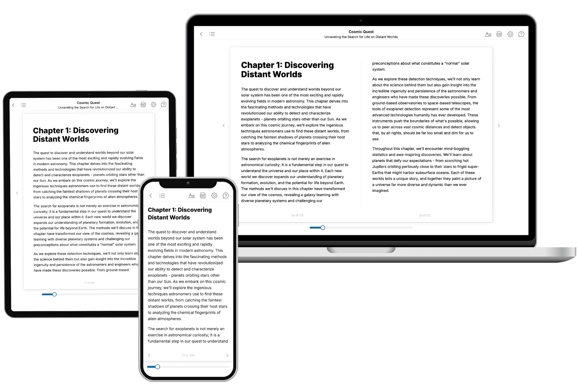
TailoredRead creates complete, full-length nonfiction ebooks, written specifically for you. Tell us what you want to learn and why, and TailoredRead writes you a complete ebook on it, with charts, tables, and diagrams throughout. Read it online, on Kindle, or on any e-reader, or download it as a PDF or EPUB. Every book is written fresh the day you order it.
- How is the book tailored to me?
Before anything is written, you answer a few short questions about your goals, your background, and the topics you care about. Your book is then planned around your answers: written at your level, focused on your goals, and covering the topics you chose, instead of the one-size-fits-all book a store sells everyone.
- Will it read like generic AI content?
No. Your book isn't a chat transcript: it's planned chapter by chapter before a single word is written, told in a clear book voice, and explains ideas visually with charts, tables, and diagrams. After writing, every book goes through an editorial pass that polishes chapters so the book reads consistent from start to finish. Judge for yourself: browse thousands of sample books on our Explore Books page.
- How accurate is the content?
Our AI first checks whether your subject needs live research. Niche and fast-moving subjects are researched before writing, and the book plan and chapters are grounded in what it finds. After writing, every book goes through a quality pass that checks its facts and consistency, and researched books list their sources in a Notes section at the back.
- How long is the book?
You choose the length: Comprehensive (250-300 pages), Detailed (150-200 pages), Essential (70-100 pages), or Short (30-50 pages).
- Does the book include visuals?
Yes. Every book includes charts, tables, and diagrams: timelines, checklists, step-by-step guides, decision trees, comparison tables, matrices, and bar charts. A typical book includes dozens of these visual elements.
- Can I read it on Kindle? What formats can I download?
Yes. Every book can be read in our online reader or downloaded as a PDF or EPUB. The EPUB can be opened with Kindle, Apple Books, Kobo, and any e-reader. The Commercial and Author licenses also include an editable Word (DOCX) and Markdown download.
- How much does it cost?
About the price of a regular ebook. The exact price depends on your book's length and complexity, from $2 for the shortest books to $35 for the most comprehensive, and it's shown when you review your book, before you commit to anything. Each book is a one-time purchase, yours to keep, no subscription. Licenses that let you share, teach, or publish your book range from $35.99 to $49.99.
- Can I preview the book before purchasing?
Before you pay, you'll see what your book will cover: the title, a detailed description, the estimated length, and the complete chapter-by-chapter table of contents, so you know what you're getting before you decide. The full text itself is written after you purchase.
- How long does it take to create a book?
About 10 minutes. You can start reading the opening chapters while the rest is still being written.