Julia for Dynamical Systems
High-Performance Computing for Chaos, Bifurcations, and Nonlinear Dynamics
Dynamical systems research demands computational power that matches the complexity of your problems.
176 pages8 chaptersAug 7, 2026Julia Programming
About this book
While Julia offers exceptional performance capabilities, translating that potential into optimized code for chaos analysis, bifurcation detection, and attractor reconstruction requires deep understanding of both the mathematics and the language's unique features. This book bridges that gap, providing expert-level guidance on implementing sophisticated dynamical systems algorithms in Julia. You'll master high-performance techniques for computing Lyapunov exponents, analyzing phase space dynamics, solving nonlinear and stochastic differential equations, and reconstructing attractors from experimental data. Each chapter combines rigorous mathematical foundations with practical Julia implementations, demonstrating how to leverage multiple dispatch, automatic differentiation, GPU acceleration, and specialized libraries to achieve research-grade performance. Whether you're investigating chaotic behavior, tracking bifurcation cascades, or reconstructing complex attractors, this book equips you with the tools and knowledge to conduct cutting-edge computational research efficiently.
Table of contents
- IntroductionWhy Julia for Dynamical Systems Research, Scope and Coverage of This Book, How to Use This Book EffectivelyRead below
- Chapter 1: Julia Fundamentals for Scientific ComputingType System and Multiple Dispatch, Performance Fundamentals and Type Stability, Profiling and Benchmarking Tools
- Chapter 2: Nonlinear Differential Equations and SolversODE Solver Methods and Selection Criteria, Adaptive Stepping and Error Control, DifferentialEquations.jl Ecosystem
- Chapter 3: Phase Space Dynamics and VisualizationPhase Space Concepts and Trajectories, Flow Analysis and Stability, Advanced Visualization Techniques
- Chapter 4: Lyapunov Exponents and Chaos QuantificationLyapunov Exponent Theory and Interpretation, Computation Methods and Algorithms, Automatic Differentiation for Sensitivity Analysis
- Chapter 5: Bifurcation Analysis and Continuation MethodsBifurcation Types and Detection, Continuation Methods and Parameter Sweeping, Bifurcation Analysis Libraries in Julia
- Chapter 6: Attractor Reconstruction from Time SeriesEmbedding Theory and Delay Coordinates, Embedding Dimension Selection Methods, Practical Reconstruction Implementation
- Chapter 7: Stochastic Differential EquationsSDE Fundamentals and Noise Models, Numerical Schemes and Convergence, Solving SDEs in Julia
- Chapter 8: Performance Optimization and GPU ComputingMemory Layout and Cache Efficiency, Parallelization Strategies, GPU Acceleration with CUDA.jl
- ConclusionIntegrating Techniques into Your Research, Future Directions in Dynamical Systems Computing
- Appendix: Code Examples and ResourcesComplete Code Examples Repository, Essential Julia Packages Reference, Further Reading and Research Resources
Introduction
Computational dynamical systems research has a measurement problem. The mathematics describing chaos, bifurcations, and attractor geometry is well-developed, but translating that mathematics into fast, reliable code has historically required painful compromises. Researchers either accepted the slow iteration cycles of interpreted languages like Python or MATLAB, or they rewrote performance-critical routines in C or Fortran and glued everything together with fragile interfaces. Neither path is satisfying when your Lyapunov spectrum computation takes hours and your parameter sweep takes days.
Julia was designed to dissolve that compromise. Its type system and multiple dispatch mechanism allow the compiler to generate specialized, optimized machine code for each concrete combination of argument types, without requiring the programmer to write separate implementations. For dynamical systems work specifically, this means that a single, readable implementation of a Runge-Kutta integrator can run at speeds competitive with hand-tuned C, while remaining composable with automatic differentiation, GPU kernels, and continuation algorithms. That composability is not incidental. It is the architectural property that makes Julia genuinely different for this class of problems.
The researchers who benefit most from this book already understand the mathematics. They know what a Poincaré section reveals about a flow, why stiff systems demand implicit solvers, and what the Kaplan-Yorke dimension measures. What they need is a precise, technically honest account of how Julia's features map onto those mathematical structures, where the performance gains are real and where they require careful setup, and how the ecosystem of specialized packages fits together into a coherent research workflow. That is exactly what this book provides.
Why Julia for Dynamical Systems Research
The case for Julia in dynamical systems research is not primarily about benchmark numbers, though those are often compelling. The deeper argument is about what becomes possible when the language's abstractions align with the mathematical structures you are working with. Dynamical systems computations are characterized by tight inner loops, heterogeneous data structures (state vectors, Jacobians, parameter arrays), and the need to compose algorithms that were developed independently. Julia's design addresses all three of these characteristics directly.
Multiple dispatch is the feature that most directly enables this composability. When you define a function in Julia, you can specialize its behavior for different combinations of argument types, and the compiler selects the most specific applicable method at compile time. For dynamical systems work, this means that an ODE solver can accept a problem definition, a Jacobian function, and a callback structure, and the compiler will generate a specialized code path for that exact combination. The result is that DifferentialEquations.jl, for example, can offer hundreds of solver algorithms through a single unified interface without sacrificing performance on any of them.[1]
Type stability is the complementary property that makes individual computations fast. A function is type-stable when the compiler can infer the output type from the input types alone, without needing to inspect runtime values. Type-unstable code forces the Julia runtime to box values and perform dynamic dispatch, which can slow execution by an order of magnitude or more. For the inner loops of Lyapunov exponent computation or ensemble integration, this difference is decisive. The chapter on Julia fundamentals covers how to write and verify type-stable code in detail, but the principle matters enough to name here: type stability is not a stylistic preference, it is a performance requirement for serious numerical work.
Julia's automatic differentiation ecosystem deserves particular attention for dynamical systems researchers. Computing Lyapunov exponents requires tracking how infinitesimal perturbations evolve under the flow, which means evaluating Jacobians of the vector field. Doing this analytically is error-prone and labor-intensive; doing it with finite differences introduces truncation error that compounds over long integrations. Julia's automatic differentiation packages can compute exact Jacobians by propagating dual numbers or adjoint sensitivities through the same code that defines the vector field, with no separate implementation required. This capability, combined with GPU acceleration through CUDA.jl, makes computations feasible that would be prohibitively slow in other environments.
A concrete comparison helps ground this. Consider computing the full Lyapunov spectrum for a 10-dimensional system over 10,000 time units, which requires integrating both the trajectory and the variational equations simultaneously. In a typical Python/NumPy implementation, the overhead of interpreted loops and repeated memory allocation makes this computation slow enough to discourage systematic parameter studies. A Julia implementation using DifferentialEquations.jl with a stiff-aware solver and in-place mutation can reduce that time by a factor of 10 to 50, depending on the system. More importantly, the Julia implementation can be extended to run as an EnsembleProblem across hundreds of parameter values in parallel, with minimal additional code.
The ecosystem maturity question is legitimate and worth addressing directly. Julia's package ecosystem for dynamical systems is now genuinely research-grade. DifferentialEquations.jl covers ODE, SDE, and delay differential equation solvers with adaptive step-size control and event handling. BifurcationKit.jl implements pseudo-arclength continuation for tracking solution branches through parameter space. Packages for delay-coordinate embedding, Lyapunov spectrum computation, and phase space visualization are actively maintained and used in published research. The ecosystem is not as large as Python's, but for the specific computational tasks that dynamical systems researchers need, the coverage is comprehensive.
There is also a practical argument about research reproducibility. Julia's package manager includes a built-in environment and manifest system that records exact package versions and their dependencies. A Julia project directory with its Project.toml and Manifest.toml files captures the complete computational environment needed to reproduce a result. For computational research where numerical results depend sensitively on solver versions and algorithm parameters, this reproducibility infrastructure is not a convenience feature. It is a scientific necessity.
| Capability | Python/NumPy | MATLAB | Julia |
|---|---|---|---|
| Execution speed (tight loops) | Slow (interpreted) | Moderate (JIT partial) | Fast (compiled via JIT) |
| ODE solver ecosystem | SciPy (limited) | Built-in (good) | DifferentialEquations.jl (extensive) |
| Automatic differentiation | JAX (separate framework) | Limited | Native, composable |
| GPU acceleration | CuPy (separate) | Partial | CUDA.jl (integrated) |
| Bifurcation continuation | PyDSTool (limited) | MatCont (external) | BifurcationKit.jl (active) |
| Reproducibility | conda/pip (fragile) | Toolbox versioning | Built-in manifest system |
| Code composability | Moderate | Low | High (multiple dispatch) |
None of this means Julia is the right tool for every task. Exploratory data analysis, figure preparation for publication, and interfacing with domain-specific experimental hardware often still favor Python or R. Julia's compilation latency on first execution (the so-called "time to first plot" problem) has improved substantially in recent versions but remains a consideration for short interactive sessions. The argument here is not that Julia dominates everywhere, but that for the specific computational core of dynamical systems research, it offers a combination of performance, composability, and mathematical expressiveness that no other language currently matches.
Scope and Coverage of This Book
This book covers the computational methods that appear most frequently in active dynamical systems research, organized around the mathematical structures they address rather than around Julia language features. Each topic is treated with enough mathematical depth to make the implementation choices meaningful, and with enough implementation detail to make the code immediately usable in research contexts. The goal is not a survey of everything Julia can do, but a precise account of how to do specific, important things well.
The foundation is Julia's type system and multiple dispatch, covered in the first chapter. Researchers coming from Python or MATLAB often underestimate how much of Julia's performance advantage flows from these two features, and how much of the ecosystem's composability depends on them. Understanding parametric types, method specialization, and type stability is not optional background knowledge. It is the prerequisite for understanding why the rest of the book's code is written the way it is. The chapter on profiling and benchmarking with BenchmarkTools.jl gives you the tools to verify that your implementations are actually achieving the performance they should.
Nonlinear differential equations and their solvers occupy the second chapter. The focus is on method selection: understanding the difference between explicit and implicit methods, recognizing stiff systems and choosing appropriate solvers, and configuring adaptive step-size control to balance accuracy against computational cost. DifferentialEquations.jl's interface is rich enough that poor configuration choices can easily negate the performance advantages of using Julia in the first place. The chapter provides concrete guidance on solver selection for the system types that appear most often in dynamical systems research.
Phase space geometry is the subject of the third chapter. Trajectories, fixed points, limit cycles, and their stability properties are the basic vocabulary of dynamical systems, and computing them accurately requires more than just integrating the equations of motion. The chapter covers how to construct phase portraits, compute Poincaré sections, and visualize high-dimensional flows in ways that reveal their geometric structure. The visualization techniques go beyond standard plotting to address the specific challenges of representing chaotic attractors and high-dimensional dynamics.
Lyapunov exponents and the Lyapunov spectrum are the subject of the fourth chapter. Computing the full spectrum requires integrating the variational equations alongside the trajectory, performing QR decompositions to prevent numerical collapse, and averaging growth rates over sufficiently long time intervals. The chapter covers both the standard algorithm and the use of automatic differentiation to compute Jacobians without manual derivation. The Kaplan-Yorke dimension, which connects the Lyapunov spectrum to the fractal dimension of the attractor, is treated as a concrete output of the computation rather than an abstract concept.
Bifurcation analysis and continuation methods occupy the fifth chapter. Tracking how a system's qualitative behavior changes as parameters vary requires more than repeated simulation at different parameter values. Pseudo-arclength continuation, as implemented in BifurcationKit.jl, can follow solution branches through fold points and detect Hopf bifurcations where fixed points lose stability to limit cycles. The chapter covers both the mathematical foundations of continuation and the practical configuration of BifurcationKit.jl for research-scale problems.
Attractor reconstruction from scalar time series is the subject of the sixth chapter. The Takens embedding theorem guarantees that a delay-coordinate embedding of a scalar observable can recover the topology of the underlying attractor, but the theorem's conditions are asymptotic and the practical implementation requires careful choices of embedding dimension and delay. The chapter covers false nearest neighbors and mutual information as dimension selection methods, and addresses the numerical challenges that arise when applying these methods to real experimental data with noise and finite length.
Stochastic differential equations are covered in the seventh chapter. The distinction between Itô calculus and Stratonovich calculus is not merely formal. It determines which numerical schemes converge to the correct solution and at what rate. The chapter covers the Euler-Maruyama method and higher-order schemes, the convergence orders relevant for different noise models, and the StochasticDiffEq.jl interface for solving SDEs with the same flexibility that DifferentialEquations.jl provides for deterministic systems.
Performance optimization and GPU computing close the technical content in the eighth chapter. Memory layout, cache efficiency, and the struct of arrays pattern are covered as concrete techniques for reducing memory bandwidth bottlenecks in large-scale simulations. The EnsembleProblem interface for parallel parameter sweeps and the CUDA.jl interface for GPU-accelerated integration are treated as practical tools with specific configuration requirements, not as aspirational capabilities.
Book Structure: From Foundations to Advanced Applications
GPU Acceleration and Performance Optimization (30)
Stochastic DEs and Attractor Reconstruction (50)
Bifurcation Analysis and Lyapunov Exponents (70)
Phase Space Dynamics and ODE Solvers (90)
Julia Fundamentals: Type System and Multiple Dispatch (110)
What this book does not cover is equally important to state clearly. It does not teach Julia as a general-purpose programming language. Readers are expected to be comfortable with basic Julia syntax, package installation, and the REPL environment before beginning. It does not cover symbolic computation, machine learning applications to dynamical systems, or control theory, though Julia has capable packages in all of these areas. The scope is deliberately narrow: the computational methods that appear most often in research on nonlinear dynamics, chaos, and bifurcations, implemented with the performance and correctness that research-grade work requires.
How to Use This Book Effectively
The chapters are ordered to build on each other, but they are not strictly sequential for readers who already have strong backgrounds in specific areas. A researcher who is comfortable with Julia's type system and already uses DifferentialEquations.jl can move directly to the chapter on Lyapunov exponents or bifurcation analysis without losing essential context. The cross-references within each chapter point to the specific concepts from earlier chapters that are being used, so you can navigate backward when needed rather than reading linearly.
The code in this book is written to be run, not just read. Every implementation is complete enough to execute in a standard Julia environment with the packages listed at the start of each chapter. The recommended approach is to work through the code interactively, modifying parameters and observing how outputs change. Dynamical systems intuition develops through experimentation, and the computational tools are most useful when you can quickly test hypotheses about how a system will behave under different conditions. Passive reading of code listings builds much less understanding than active modification and re-execution.
Setting up your environment correctly before starting will save significant frustration. The following steps establish a clean, reproducible workspace:
Setting Up Your Julia Research Environment
- Install Julia - Download the current stable release from julialang.org. As of this writing, Julia 1.10 or later is recommended for the packages used in this book. Avoid using system package managers for Julia itself, as they often provide outdated versions.
- Create a project directory - For each research project or book chapter, create a dedicated directory and activate a new Julia environment inside it using `julia --project=.` or by running `] activate .` in the REPL. This isolates package versions per project.
- Install core packages - Add DifferentialEquations.jl, BenchmarkTools.jl, and a plotting package (Makie.jl is recommended for dynamical systems visualization) to your environment. Use `] add PackageName` in the REPL package manager mode.
- Verify type stability tooling - Install the Cthulhu.jl package for interactive type inference inspection. Run `@code_warntype` on your key functions before benchmarking to catch type instabilities early.
- Configure parallel computing - Set the JULIA_NUM_THREADS environment variable before starting Julia to enable multi-threading. For GPU work, install CUDA.jl and verify that your CUDA toolkit version is compatible with the installed package version.
- Test your setup - Run a simple Lorenz system integration using DifferentialEquations.jl and verify that the solution completes without errors and that BenchmarkTools.jl reports timing in the expected range for your hardware.
Each chapter includes benchmark results for the implementations it presents. These numbers were obtained on specific hardware configurations, and your results will differ based on your CPU, memory bandwidth, and GPU if applicable. The absolute numbers matter less than the relative comparisons: how much faster is the type-stable version than the type-unstable version, how much does in-place mutation reduce allocation overhead, how does GPU acceleration scale with problem size. Focus on understanding the sources of performance differences rather than matching specific timing figures.
The mathematical notation in this book follows conventions standard in the dynamical systems literature. State vectors are bold lowercase letters (x), parameter vectors are bold Greek letters, and the flow map is denoted φ. Jacobians are denoted Df for the derivative of the vector field f. Where Julia code uses different variable names for practical reasons (Julia convention favors short names in tight loops), the correspondence between mathematical notation and code variables is made explicit. This dual notation is intentional: the goal is to keep the connection between the mathematics and the implementation visible throughout.
Common pitfalls appear throughout the text as explicit warnings rather than being buried in footnotes. Type instabilities that are easy to introduce accidentally, solver configurations that silently produce inaccurate results, and embedding parameter choices that lead to spurious dimension estimates are all flagged at the point where they are most likely to occur. The warnings are specific: not "be careful with numerical precision" but "using Float32 for Lyapunov exponent computation will cause the QR decomposition to lose orthogonality after approximately N steps for typical chaotic systems."
The relationship between chapters reflects the structure of actual research workflows. A typical dynamical systems study might begin with ODE integration to characterize the system's behavior, proceed to phase space visualization to identify interesting parameter regimes, use bifurcation continuation to map out the parameter space systematically, and then compute Lyapunov exponents to quantify chaos in the identified regimes. The chapter ordering follows this natural progression. When a later chapter uses a technique from an earlier one, it references the earlier chapter by the concept it covers rather than by chapter number, so the logical dependencies are clear even if you are reading non-sequentially.
For researchers who are new to Julia but experienced in dynamical systems, the first chapter deserves careful attention even if it feels like it covers familiar ground. The specific ways that Julia's type system differs from Python's duck typing or MATLAB's dynamic typing have concrete consequences for how you structure numerical code, and those consequences appear throughout the rest of the book. Spending time with the profiling and benchmarking tools in that chapter will also give you a reliable way to verify that your implementations are performing as expected, which is more valuable than any specific optimization technique.
For researchers who are experienced Julia programmers but newer to dynamical systems, the mathematical context provided at the start of each chapter is intended to be self-contained enough to make the computational choices meaningful. The goal is not to replace a textbook on nonlinear dynamics, but to provide enough mathematical grounding that the implementation decisions make sense on their own terms. References to standard texts are provided for readers who want deeper mathematical treatment of specific topics.
Where to Start Based on Your Background
- What is your primary background?
- Strong Julia, newer to dynamical systems Start with the chapter on ODE solvers and DifferentialEquations.jl
- Strong dynamical systems, newer to Julia Start with the Julia fundamentals chapter, focusing on type stability and BenchmarkTools.jl
- Expert in both areas Begin with the chapter on Lyapunov exponents or bifurcation analysis, referencing earlier chapters as needed
- Building both skills simultaneously Work through the Julia fundamentals chapter first, then follow the chapters in order
The appendix contains a complete package reference with version information, a curated list of further reading organized by topic, and a repository of complete code examples that can be used as starting points for research implementations. The code repository is organized to mirror the chapter structure, so finding the complete implementation of any algorithm discussed in the text is straightforward. Where the in-chapter code presents simplified versions for clarity, the appendix versions include the full error handling, parameter validation, and output formatting that production research code requires.
One practical note on Julia's compilation behavior: the first time you run any function in a Julia session, the compiler generates specialized machine code for the argument types you provide. This compilation takes time, sometimes several seconds for complex functions. Subsequent calls with the same argument types execute the compiled code directly and are fast. This means that benchmarks should always be run after a warm-up call, and that the timing you experience in interactive use will improve after the first execution. BenchmarkTools.jl handles this automatically by running multiple trials, but it is worth understanding the underlying mechanism so that slow first-run times do not create a misleading impression of Julia's steady-state performance. The research workflows described in this book are designed around this compilation model, and the performance characteristics discussed throughout assume compiled, steady-state execution.
Notes
Introduction
- 1. Christopher Rackauckas and Qing Nie, "DifferentialEquations.jl - A Performant and Feature-Rich Ecosystem for Solving Differential Equations in Julia," Journal of Open Research Software, 2017
This is the end of the free sample. The full book has 8 chapters.
Want this book written for you?
Tell us your goals and background, and get your own version of this book, tailored by AI to you.


Benefits of AI-tailored books
- Read one book, not ten:
- all the Julia Programming knowledge you need, gathered into a single book.
- Save days of learning:
- tell us your goals, choose your topics, and the whole book is built around them.
- Learn effortlessly:
- Julia Programming book written for your specific background and expertise.
- Understand at a glance:
- includes charts, tables, timelines, checklists, decision trees, and more.
- Stay current:
- written the day you order it, not years ago.
- Trust what you read:
- every book is checked for accuracy, with real research when your subject needs it.
Create your unique book in 3 steps
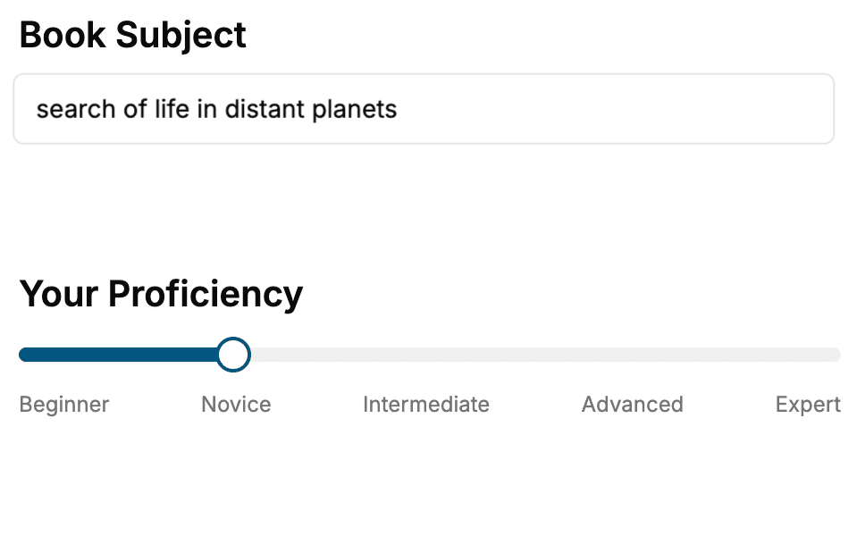
- 1. Select your focus
Select the focus of your Julia Programming book and share your background
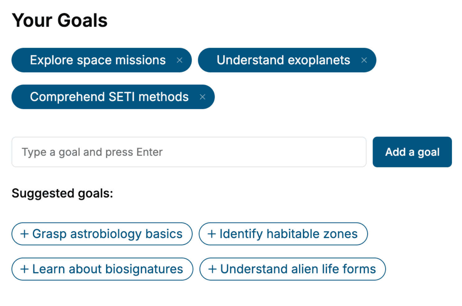
- 2. Personalize your book
Specify your goals and choose sub-topics to include
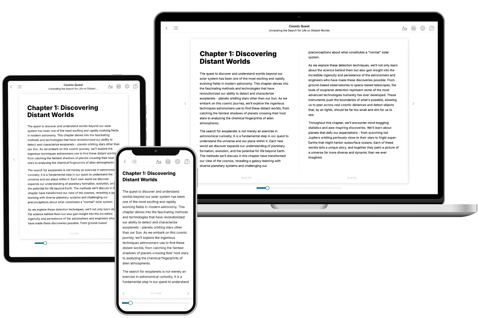
- 3. Get your tailored book
Your book is ready in 10 minutes. Read it online, download as EPUB or PDF, or send to Kindle.
Frequently asked questions
- What is TailoredRead?
TailoredRead creates complete, full-length nonfiction ebooks, written specifically for you. Tell us what you want to learn and why, and TailoredRead writes you a complete ebook on it, with charts, tables, and diagrams throughout. Read it online, on Kindle, or on any e-reader, or download it as a PDF or EPUB. Every book is written fresh the day you order it.
- How is the book tailored to me?
Before anything is written, you answer a few short questions about your goals, your background, and the topics you care about. Your book is then planned around your answers: written at your level, focused on your goals, and covering the topics you chose, instead of the one-size-fits-all book a store sells everyone.
- Will it read like generic AI content?
No. Your book isn't a chat transcript: it's planned chapter by chapter before a single word is written, told in a clear book voice, and explains ideas visually with charts, tables, and diagrams. After writing, every book goes through an editorial pass that polishes chapters so the book reads consistent from start to finish. Judge for yourself: browse thousands of sample books on our Explore Books page.
- How accurate is the content?
Our AI first checks whether your subject needs live research. Niche and fast-moving subjects are researched before writing, and the book plan and chapters are grounded in what it finds. After writing, every book goes through a quality pass that checks its facts and consistency, and researched books list their sources in a Notes section at the back.
- How long is the book?
You choose the length: Comprehensive (250-300 pages), Detailed (150-200 pages), Essential (70-100 pages), or Short (30-50 pages).
- Does the book include visuals?
Yes. Every book includes charts, tables, and diagrams: timelines, checklists, step-by-step guides, decision trees, comparison tables, matrices, and bar charts. A typical book includes dozens of these visual elements.
- Can I read it on Kindle? What formats can I download?
Yes. Every book can be read in our online reader or downloaded as a PDF or EPUB. The EPUB can be opened with Kindle, Apple Books, Kobo, and any e-reader. The Commercial and Author licenses also include an editable Word (DOCX) and Markdown download.
- How much does it cost?
About the price of a regular ebook. The exact price depends on your book's length and complexity, from $2 for the shortest books to $35 for the most comprehensive, and it's shown when you review your book, before you commit to anything. Each book is a one-time purchase, yours to keep, no subscription. Licenses that let you share, teach, or publish your book range from $35.99 to $49.99.
- Can I preview the book before purchasing?
Before you pay, you'll see what your book will cover: the title, a detailed description, the estimated length, and the complete chapter-by-chapter table of contents, so you know what you're getting before you decide. The full text itself is written after you purchase.
- How long does it take to create a book?
About 10 minutes. You can start reading the opening chapters while the rest is still being written.