Climate Modeling Essentials
Mastering Numerical Algorithms and Computational Methods for Earth System Simulation
Most people think climate models are black boxes that simply predict future temperatures.
207 pages9 chaptersMay 18, 2026Climate Change
About this book
In reality, they're sophisticated computational systems built on decades of numerical algorithm research. This book demystifies the mathematical and computational foundations that make climate modeling possible. You'll discover how scientists discretize Earth's complex fluid dynamics equations into solvable computational problems, why certain numerical methods work better than others for different climate phenomena, and how modern supercomputers enable global simulations. Whether you're a student entering the field, a professional seeking deeper technical understanding, or a researcher looking to implement or improve climate models, this guide provides the practical knowledge you need. From grid design and time-stepping schemes to parameterization strategies and parallel computing approaches, you'll gain insight into the real engineering decisions that shape climate predictions and their uncertainties.
Table of contents
- IntroductionWhy Climate Modeling Matters, The Computational Challenge, What You'll Learn in This Book, How to Use This GuideRead below
- Chapter 1: Foundations of Climate EquationsThe Governing Equations of Fluid Dynamics, Navier-Stokes and Primitive Equations, Thermodynamic and Conservation Equations
- Chapter 2: Discretization and Grid DesignSpatial Discretization Fundamentals, Grid Types and Staggering Strategies, Resolution Trade-offs and Computational Cost
- Chapter 3: Finite Difference MethodsFinite Difference Basics and Taylor Series, Accuracy Orders and Truncation Error, Applications in Climate Models
- Chapter 4: Finite Element and Spectral MethodsFinite Element Method Principles, Spectral Methods and Fourier Analysis, Comparing Methods for Climate Applications
- Chapter 5: Time-Stepping Schemes and StabilityExplicit Time-Stepping Methods, Implicit and Semi-Implicit Methods, Stability Analysis and the CFL Condition
- Chapter 6: Parameterization and Sub-Grid ProcessesThe Parameterization Problem, Convection and Cloud Parameterization, Turbulence and Boundary Layer Schemes
- Chapter 7: Parallel Computing and ScalabilityParallel Computing Fundamentals, Domain Decomposition Strategies, Performance Optimization and Load Balancing
- Chapter 8: Validation, Uncertainty, and Error AnalysisModel Validation and Benchmarking, Uncertainty Quantification Methods, Sources of Error and Limitations
- Chapter 9: Practical Implementation and ToolsClimate Modeling Software Frameworks, Implementation Strategies and Best Practices, Debugging and Performance Profiling
- ConclusionKey Takeaways, Future Directions in Climate Modeling
- Glossary
- Further Reading and Resources
Introduction
Every weather forecast you check on your phone, every projection about sea level rise, and every policy debate about carbon emissions ultimately traces back to the same source: numerical climate models running on some of the most powerful computers ever built. These models are not simple extrapolations or educated guesses. They are sophisticated computational systems that encode the fundamental laws of physics, chemistry, and fluid dynamics into millions of lines of code, then solve those equations across billions of grid points spanning the entire planet. Understanding how they work is no longer optional for anyone serious about climate science or Earth system research.
The gap between knowing that climate models exist and understanding how they actually function is surprisingly wide. Most introductory courses in climate science focus on the physical processes: the greenhouse effect, ocean circulation, ice-albedo feedback. That knowledge is essential, but it leaves out the computational machinery that makes simulation possible in the first place. How do you turn a continuous differential equation describing atmospheric flow into something a computer can actually calculate? How do you decide how fine to make your grid? How do you keep numerical errors from growing until they swamp your signal? These are engineering questions as much as scientific ones, and they have real consequences for the reliability of climate predictions.
This book was written for people who already have some footing in both climate science and computer science, and who want to connect those two worlds more deeply. You do not need to be an expert in either field, but you should be comfortable with calculus, basic linear algebra, and at least one programming language. The goal is not to turn you into a climate model developer overnight. The goal is to give you a clear, practical understanding of the numerical algorithms and computational methods that underpin modern Earth system simulation, so you can read the literature more critically, contribute to modeling projects more effectively, and make better decisions about how to use and interpret model output.
The chapters ahead move from foundations to applications in a deliberate sequence. You will start with the governing equations of fluid dynamics and thermodynamics, then work through discretization strategies, numerical methods, time-stepping schemes, parameterization, parallel computing, and validation. Each topic builds on the previous one. By the end, you will have a coherent picture of how a global climate model is assembled from mathematical principles all the way through to running on a supercomputer and producing output that scientists and policymakers actually use.
Why Climate Modeling Matters
Climate modeling sits at the intersection of some of the most consequential scientific and policy questions of our time. The projections produced by models like those in the Coupled Model Intercomparison Project (CMIP) directly inform the reports of the Intergovernmental Panel on Climate Change (IPCC), which in turn shape international agreements, national energy policies, and infrastructure investment decisions worth trillions of dollars.[1] When a government decides how high to build a coastal flood barrier, or how aggressively to pursue emissions reductions, climate model output is part of that calculation. The stakes are not abstract.
Beyond policy, climate models are indispensable scientific tools. They allow researchers to run controlled experiments that are impossible in the real world. You cannot remove all the CO₂ from the atmosphere to test its effect, but you can do exactly that in a model. You can isolate the contribution of volcanic eruptions to historical temperature changes, test hypotheses about past ice ages, or explore how different land-use patterns affect regional precipitation. This experimental capability has made climate models central to advancing our understanding of Earth's climate system in ways that observation alone cannot achieve.
The practical applications extend well beyond long-term climate projection. Numerical weather prediction, which shares much of its mathematical foundation with climate modeling, now produces forecasts accurate enough to save lives during extreme weather events. Seasonal forecasting helps agricultural planners prepare for drought or flood conditions months in advance. Ocean models guide shipping routes and fisheries management. The same computational methods you will learn in this book power all of these applications, which means the knowledge transfers broadly across Earth system science.
It is also worth being honest about what climate models cannot do. They are not crystal balls. Every model contains approximations, and every projection carries uncertainty. Understanding the computational foundations of climate modeling is partly about appreciating the power of these tools, but it is equally about understanding their limitations. A researcher who knows how parameterization schemes work, for example, is far better equipped to interpret the spread in model projections than one who treats model output as a black box. Critical engagement with climate models requires technical literacy, and that is exactly what this book aims to build.
The history of climate modeling is also a story of remarkable scientific progress driven by computational innovation. The first general circulation model (GCM) was developed by Norman Phillips at Princeton in 1956, running on a computer that occupied an entire room and could barely simulate two weeks of atmospheric flow.[2] Today's Earth system models simulate centuries of climate across the entire globe, including atmosphere, ocean, land surface, sea ice, and biogeochemical cycles, running on machines with hundreds of thousands of processor cores. That progression did not happen by accident. It happened because generations of scientists and engineers solved hard numerical and computational problems, one algorithm at a time.
Understanding that history gives context to the choices embedded in modern models. Many of the numerical methods used today were developed decades ago and carry design decisions shaped by the hardware of their era. Some of those decisions are still optimal; others are legacy constraints that the field is actively working to move beyond. Knowing the difference requires understanding the underlying algorithms, which is another reason why the computational foundations covered in this book matter so much for anyone working in or adjacent to climate science.
Climate models are not predictions of the future. They are tools for exploring what the future could look like under different assumptions, and their value depends entirely on how well we understand what goes into them.
The Computational Challenge
To appreciate why climate modeling is computationally demanding, consider what you are actually trying to simulate. The atmosphere alone is a turbulent fluid covering the entire planet, extending roughly 100 kilometers upward, driven by solar radiation, rotating with the Earth, and interacting continuously with the ocean, land surface, and cryosphere. The equations that govern this fluid, the Navier-Stokes equations combined with thermodynamic and tracer transport equations, are nonlinear partial differential equations with no general analytical solution. The only way to solve them for realistic conditions is numerically, which means discretizing them onto a grid and solving them step by step through time.
The scale of that discretization problem is staggering. A modern high-resolution global atmosphere model might use a horizontal grid spacing of 25 kilometers, which requires roughly 500,000 horizontal grid columns. With 100 vertical levels, that gives 50 million grid points in the atmosphere alone. At each grid point, the model tracks a dozen or more variables: temperature, pressure, wind components, humidity, and various chemical tracers. At each time step, which might be as short as 10 minutes for stability reasons, the model must update all of those variables by solving the discretized equations. Running a 100-year climate simulation at that resolution requires on the order of 1018 floating-point operations, which is why climate models run on supercomputers rather than laptops.[3]
The challenge is not just raw computational power. It is also about numerical accuracy and stability. Climate simulations run for decades or centuries of simulated time, which means numerical errors can accumulate over millions of time steps. A small error in the discretization scheme that grows by even a tiny fraction each step can eventually dominate the solution. This is why the choice of numerical method matters so much. Different methods have different accuracy properties, different stability characteristics, and different computational costs, and the right choice depends on the specific equations and phenomena being simulated.
There is also the challenge of scale separation. Climate-relevant processes span an enormous range of spatial and temporal scales. Large-scale atmospheric circulation patterns operate at thousands of kilometers and evolve over weeks. Individual convective clouds operate at kilometers and evolve over minutes. Ocean eddies operate at tens of kilometers and persist for weeks. No single grid can resolve all of these scales simultaneously at global extent, at least not with current computing resources. This forces modelers to make explicit choices about what to resolve and what to approximate, which is the parameterization problem that occupies an entire chapter of this book.
Memory and data management add another layer of complexity. A single time step of a high-resolution Earth system model can generate gigabytes of data. A full simulation produces terabytes or petabytes of output that must be stored, transferred, and analyzed. The computational infrastructure required to support climate modeling extends well beyond the model code itself, encompassing storage systems, data pipelines, visualization tools, and analysis frameworks. Understanding the computational challenge means understanding this entire ecosystem, not just the numerical algorithms at its core.
Parallel computing is the primary tool for managing this complexity. Modern climate models distribute their grid across hundreds or thousands of processor cores, with each core responsible for a subdomain of the global grid. This domain decomposition approach allows the computation to scale with available hardware, but it introduces its own challenges around communication overhead, load balancing, and synchronization. Getting good parallel performance from a climate model requires careful attention to both the numerical algorithms and the software architecture, which is why parallel computing gets dedicated coverage later in this book.
One concrete illustration of the computational challenge: the European Centre for Medium-Range Weather Forecasts (ECMWF) runs its operational forecast model at a horizontal resolution of about 9 kilometers globally. A single 10-day forecast requires roughly 1016 floating-point operations and takes about an hour on a machine with tens of thousands of cores.[4] Climate models running century-long simulations face even greater demands, which is why the computational methods used to build them represent some of the most sophisticated numerical engineering in applied science.
The good news is that the core ideas behind these methods are accessible. You do not need to understand every detail of a production climate model to grasp the principles that make it work. The chapters ahead break down these principles into manageable pieces, starting from the mathematical foundations and building up to the full computational system. Each piece is explained in terms of the problem it solves and the trade-offs it involves, so you can develop genuine intuition rather than just surface familiarity.
What You'll Learn in This Book
This book covers the full computational stack of climate modeling, from the governing equations at the top to parallel computing infrastructure at the bottom. The coverage is organized to build understanding progressively, with each chapter providing the foundation for the ones that follow. Here is a brief map of what each chapter covers and why it matters.
Chapter 1: Foundations of Climate Equations starts with the physics. Before you can discretize equations, you need to understand what those equations are and where they come from. This chapter covers the Navier-Stokes equations, the primitive equations used in most atmospheric models, and the thermodynamic and conservation equations that govern temperature, moisture, and chemical tracers. The focus is on building physical intuition for what each term in these equations represents, because that intuition is essential for making good numerical choices later.
Chapter 2: Discretization and Grid Design addresses the fundamental step of converting continuous equations into discrete computational problems. You will learn about different grid types, including regular latitude-longitude grids, cubed-sphere grids, and unstructured meshes, and understand the trade-offs each involves. The chapter also covers grid staggering strategies, which determine how different variables are positioned relative to each other on the grid, and explains why these choices affect both accuracy and stability.
Chapters 3 and 4 cover the three main families of spatial discretization methods used in climate models:
- Finite difference methods (Chapter 3): the most intuitive approach, based on approximating derivatives using differences between neighboring grid points. You will learn about accuracy orders, truncation error, and how these methods are applied to specific climate model equations.
- Finite element methods (Chapter 4): a more flexible approach that works well on unstructured grids and handles complex geometries. You will learn the variational principles behind FEM and see how they are applied in modern atmospheric dynamical cores.
- Spectral methods (Chapter 4): an approach based on representing fields as sums of basis functions, offering very high accuracy for smooth problems. You will learn why spectral methods dominated atmospheric modeling for decades and why some models are moving away from them.
Chapter 5: Time-Stepping Schemes and Stability covers the temporal dimension of the numerical problem. Spatial discretization gives you a system of ordinary differential equations in time; time-stepping schemes determine how you advance that system forward. You will learn about explicit methods like Runge-Kutta, implicit methods that require solving linear systems at each step, and semi-implicit approaches that treat different terms differently to balance accuracy and stability. The chapter also covers the Courant-Friedrichs-Lewy (CFL) condition, the fundamental stability constraint that determines how small your time step must be relative to your grid spacing.
Chapter 6: Parameterization and Sub-Grid Processes addresses one of the most scientifically important and technically challenging aspects of climate modeling. Because no grid can resolve all relevant scales, processes smaller than the grid spacing must be represented through parameterization schemes that relate sub-grid effects to resolved-scale variables. You will learn how convection, clouds, turbulence, and boundary layer processes are parameterized, and understand why parameterization uncertainty is one of the largest sources of spread in climate projections.
Chapter 7: Parallel Computing and Scalability covers the computational infrastructure that makes global climate simulation possible. You will learn about domain decomposition strategies, message-passing interfaces, and the performance trade-offs involved in scaling a climate model across thousands of processor cores. The chapter also addresses load balancing challenges that arise when different parts of the model have different computational costs, such as when sea ice is present in some grid columns but not others.
Chapter 8: Validation, Uncertainty, and Error Analysis addresses the critical question of how much you can trust model output. You will learn about model validation strategies, including comparison with observations and reanalysis products, and about formal methods for quantifying uncertainty in climate projections. The chapter also provides a systematic taxonomy of error sources, from numerical truncation errors to structural model errors, so you can reason clearly about where uncertainty comes from and how it propagates through a simulation.
Chapter 9: Practical Implementation and Tools brings everything together in a practical context. You will learn about the major climate modeling software frameworks, including the Community Earth System Model (CESM) and the Model for Prediction Across Scales (MPAS), and get guidance on implementation strategies, debugging approaches, and performance profiling techniques. This chapter is designed to help you move from understanding the concepts to actually working with real climate model code.
By the end of this book, you will be able to read a climate model technical description and understand the numerical choices being made. You will be able to evaluate the trade-offs between different discretization approaches, understand why a particular time-stepping scheme was chosen, and interpret parameterization uncertainty in model projections. You will also have a practical foundation for contributing to climate modeling projects, whether that means implementing a new parameterization scheme, optimizing parallel performance, or designing a validation experiment.
How to Use This Guide
This book is designed to be read sequentially, because each chapter builds on concepts introduced in earlier ones. If you skip directly to the chapter on parallel computing without reading the chapters on discretization and time-stepping, you will miss the context that makes the parallel computing choices meaningful. That said, the book is also structured so that individual chapters can serve as reference material once you have read through it once. Each chapter is self-contained enough to be revisited independently when you need a refresher on a specific topic.
The assumed background is intermediate level. Specifically, you should be comfortable with:
- Multivariable calculus, including partial derivatives and the divergence theorem
- Basic linear algebra, including matrix operations and eigenvalue concepts
- Ordinary and partial differential equations at an introductory level
- At least one programming language, preferably Python, Fortran, or C/C++
- Introductory climate science, including the basic structure of the atmosphere and ocean
Mathematical notation is used throughout the book, but the emphasis is always on intuition and practical understanding rather than formal rigor. When an equation appears, it is accompanied by an explanation of what each term means physically and why it matters computationally. The goal is never to impress with mathematical sophistication but to give you the tools to reason clearly about numerical problems. If you find yourself getting lost in the math, focus on the surrounding explanation and come back to the equations once the conceptual picture is clear.
Code examples appear in several chapters, particularly in the later chapters on implementation and tools. These examples are written primarily in Python for accessibility, with notes on how the same concepts apply in Fortran or C++, which are the languages most commonly used in production climate models. The code is meant to illustrate concepts, not to serve as production-ready implementations. Treat it as a starting point for your own exploration rather than a template to copy directly into a real model.
Each chapter ends with a set of practical exercises designed to reinforce the concepts covered. These range from analytical problems, such as deriving the truncation error of a finite difference scheme, to computational exercises, such as implementing a simple advection scheme and testing its stability properties. Working through these exercises is strongly recommended. Climate modeling is a hands-on discipline, and the concepts in this book become much more concrete once you have implemented them yourself, even in simplified form.
For those using this book in a course or study group, the chapter structure maps naturally onto a semester-length curriculum. Chapters 1 through 5 cover the core numerical methods and could form the first half of a course, while Chapters 6 through 9 cover more advanced and applied topics suitable for the second half. The introduction and conclusion provide framing that works well for the first and last sessions of a course. Instructors are encouraged to supplement the exercises with real model output analysis, which helps connect the abstract numerical concepts to the actual behavior of climate simulations.
A note on notation: this book uses standard mathematical conventions throughout. Vectors are denoted in bold (for example, u for the velocity vector), scalars in italic (for example, T for temperature), and operators in upright font (for example, ∇ for the gradient operator). Subscripts denote spatial indices and superscripts denote time levels, so Ti,jn refers to the temperature at grid point (i,j) at time step n. This notation is consistent with most of the climate modeling literature, so getting comfortable with it here will help you read primary sources more easily.
Finally, approach this material with patience and curiosity. Climate modeling sits at the frontier of applied mathematics, computational science, and Earth system science, and it is genuinely difficult. Some of the concepts, particularly around numerical stability and parameterization, took the research community decades to work out. You are not expected to master everything on a first reading. The goal is to build a solid foundation that you can continue to develop through practice, reading, and engagement with real modeling problems. The field needs people who understand both the science and the computation, and this book is designed to help you become one of them.
The best way to understand a climate model is to build one, even a simple one. Every concept in this book becomes clearer the moment you implement it in code and watch it either work correctly or fail in an instructive way.
Notes
Introduction
- 1. IPCC, 2021: Climate Change 2021: The Physical Science Basis. Contribution of Working Group I to the Sixth Assessment Report of the Intergovernmental Panel on Climate Change. Cambridge University Press.
- 2. N. A. Phillips, "The general circulation of the atmosphere," Quarterly Journal of the Royal Meteorological Society, 1956
- 3. V. Balaji and others, "CPMIP: measurements of real computational performance of Earth system models in CMIP6," Geoscientific Model Development, 2017
- 4. ECMWF, IFS Documentation CY48R1, European Centre for Medium-Range Weather Forecasts, 2023
This is the end of the free sample. The full book has 9 chapters.
Want this book written for you?
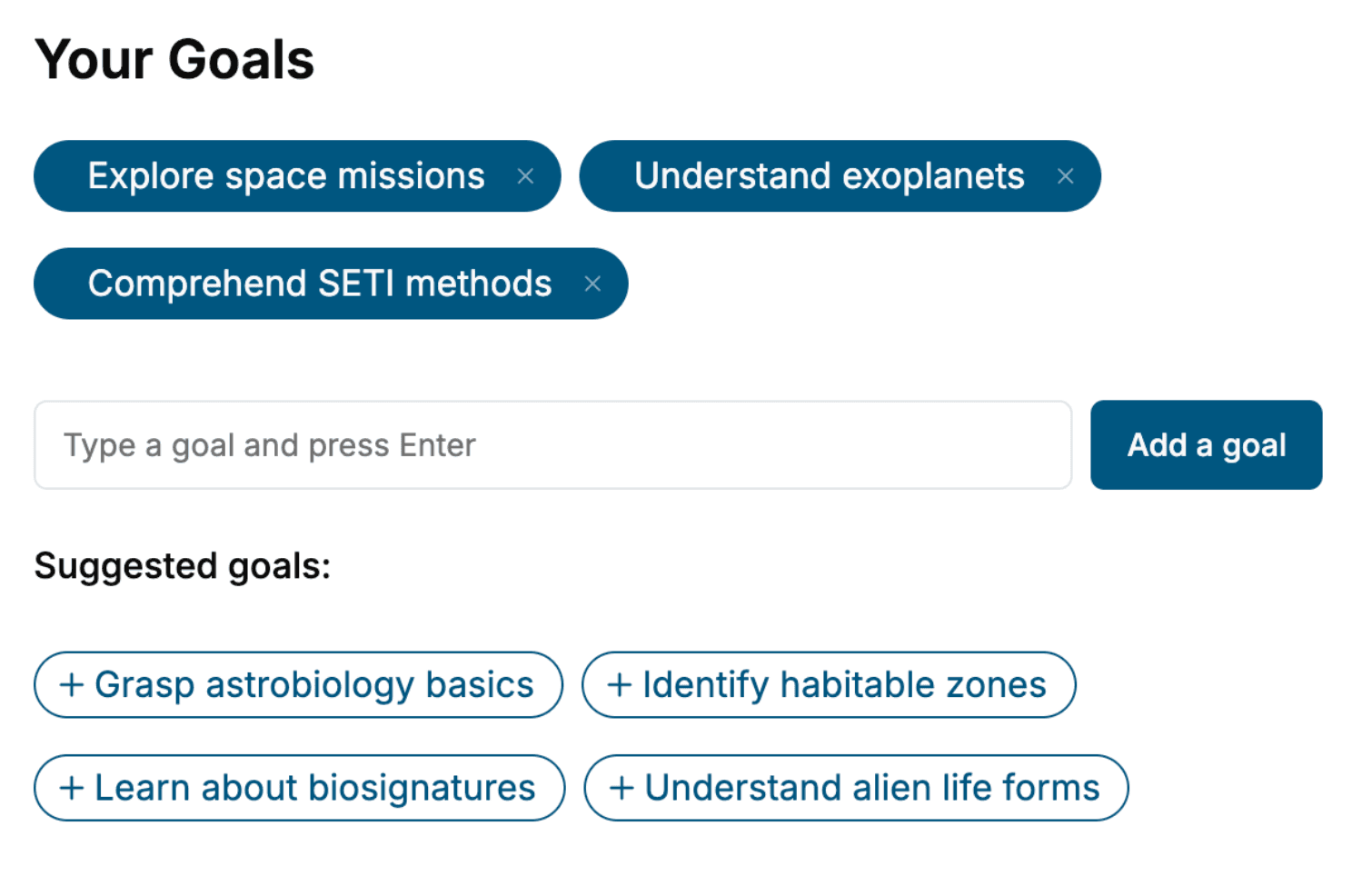
Tell us your goals and background, and get your own version of this book, tailored by AI to you.


Benefits of AI-tailored books
- Read one book, not ten:
- all the Climate Change knowledge you need, gathered into a single book.
- Save days of learning:
- tell us your goals, choose your topics, and the whole book is built around them.
- Learn effortlessly:
- Climate Change book written for your specific background and expertise.
- Understand at a glance:
- includes charts, tables, timelines, checklists, decision trees, and more.
- Stay current:
- written the day you order it, not years ago.
- Trust what you read:
- every book is checked for accuracy, with real research when your subject needs it.
Create your unique book in 3 steps
- 1. Select your focus
Select the focus of your Climate Change book and share your background
- 2. Personalize your book
Specify your goals and choose sub-topics to include
- 3. Get your tailored book
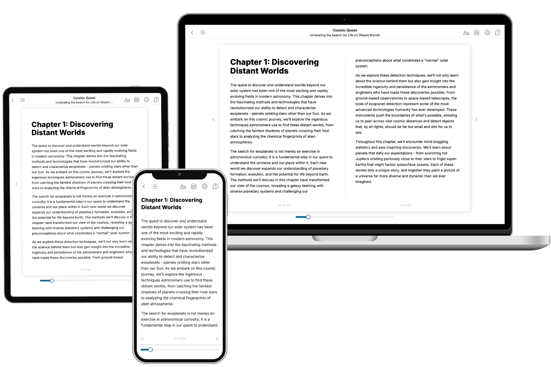
Your book is ready in 10 minutes. Read it online, download as EPUB or PDF, or send to Kindle.

Frequently asked questions
- What is TailoredRead?
TailoredRead creates complete, full-length nonfiction ebooks, written specifically for you. Tell us what you want to learn and why, and TailoredRead writes you a complete ebook on it, with charts, tables, and diagrams throughout. Read it online, on Kindle, or on any e-reader, or download it as a PDF or EPUB. Every book is written fresh the day you order it.
- How is the book tailored to me?
Before anything is written, you answer a few short questions about your goals, your background, and the topics you care about. Your book is then planned around your answers: written at your level, focused on your goals, and covering the topics you chose, instead of the one-size-fits-all book a store sells everyone.
- Will it read like generic AI content?
No. Your book isn't a chat transcript: it's planned chapter by chapter before a single word is written, told in a clear book voice, and explains ideas visually with charts, tables, and diagrams. After writing, every book goes through an editorial pass that polishes chapters so the book reads consistent from start to finish. Judge for yourself: browse thousands of sample books on our Explore Books page.
- How accurate is the content?
Our AI first checks whether your subject needs live research. Niche and fast-moving subjects are researched before writing, and the book plan and chapters are grounded in what it finds. After writing, every book goes through a quality pass that checks its facts and consistency, and researched books list their sources in a Notes section at the back.
- How long is the book?
You choose the length: Comprehensive (250-300 pages), Detailed (150-200 pages), Essential (70-100 pages), or Short (30-50 pages).
- Does the book include visuals?
Yes. Every book includes charts, tables, and diagrams: timelines, checklists, step-by-step guides, decision trees, comparison tables, matrices, and bar charts. A typical book includes dozens of these visual elements.
- Can I read it on Kindle? What formats can I download?
Yes. Every book can be read in our online reader or downloaded as a PDF or EPUB. The EPUB can be opened with Kindle, Apple Books, Kobo, and any e-reader. The Commercial and Author licenses also include an editable Word (DOCX) and Markdown download.
- How much does it cost?
About the price of a regular ebook. The exact price depends on your book's length and complexity, from $2 for the shortest books to $35 for the most comprehensive, and it's shown when you review your book, before you commit to anything. Each book is a one-time purchase, yours to keep, no subscription. Licenses that let you share, teach, or publish your book range from $35.99 to $49.99.
- Can I preview the book before purchasing?
Before you pay, you'll see what your book will cover: the title, a detailed description, the estimated length, and the complete chapter-by-chapter table of contents, so you know what you're getting before you decide. The full text itself is written after you purchase.
- How long does it take to create a book?
About 10 minutes. You can start reading the opening chapters while the rest is still being written.